Texas planters got wealthy in the 1850s because they combined three things that rarely line up so perfectly: nearly unlimited cheap land suited for cotton, a growing enslaved labor force that kept production costs low, and a global cotton market that was hungry for every bale they could ship. Cotton output in Texas exploded from roughly 58,073 bales in 1849 to over 431,645 bales by 1859, a more than sevenfold increase in a single decade. That kind of growth, built on a crop that could be grown, ginned, and sold through established trade routes, turned a handful of well-positioned planters into some of the wealthiest people in the antebellum South.
Why Texas Planters Grew Wealthy in the 1850s

Samuel Rourke
1 Jul 2026
Texas agriculture in the 1850s: the big picture
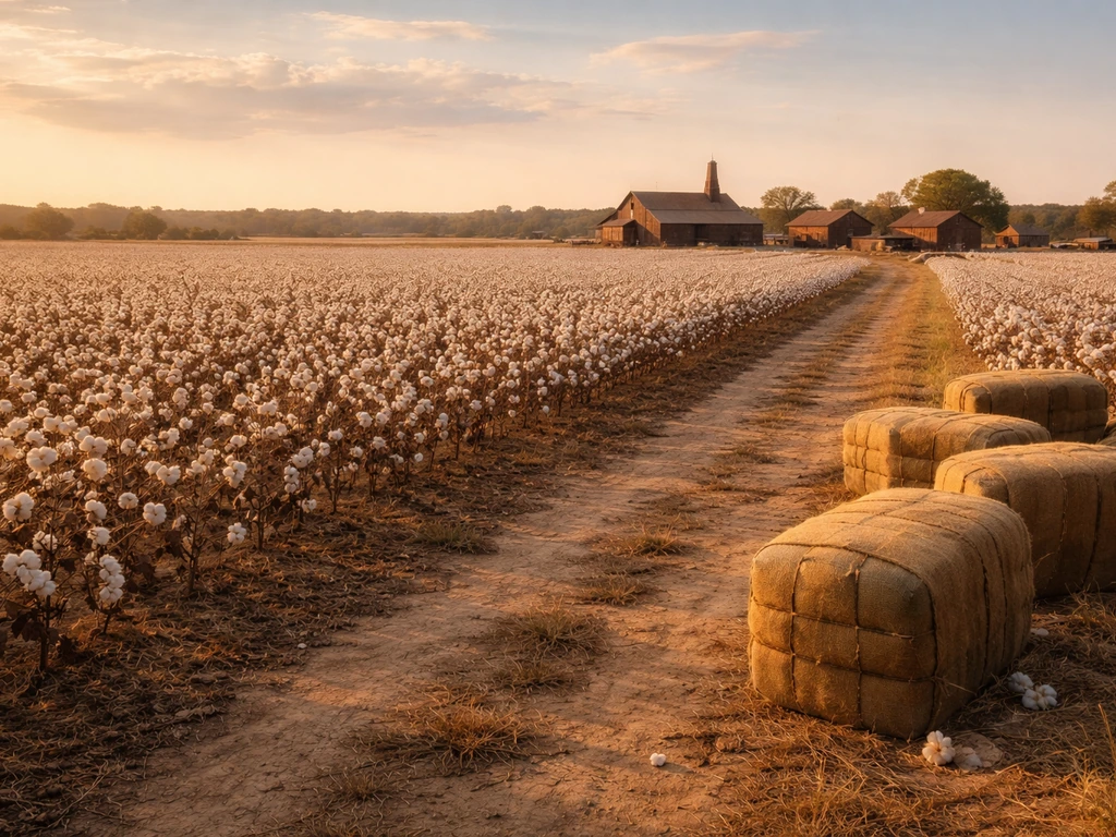
When Texas entered the Union in 1845, its agricultural economy was still finding its footing. But by the early 1850s, the plantation districts were taking shape fast. The river bottoms of the Brazos, Colorado, and Trinity river corridors in south-central Texas became the heartland of commercial cotton farming. These weren't small family plots. They were large operations engineered to maximize cotton output, and the 1850s gave planters every structural advantage they needed to scale up quickly.
The decade also saw significant territorial expansion within the state. As Indian tribes were pushed out of previously contested lands, new acreage opened up for cultivation, and planters who could afford to act quickly snapped it up. That land opening is one of the factors TSHA directly credits for the sharp rise in late-1850s cotton yields. By the time the 1860 census was counted, Texas had transformed from a frontier agricultural state into a significant cotton-producing powerhouse.
What crops made money, and why cotton fit Texas so well
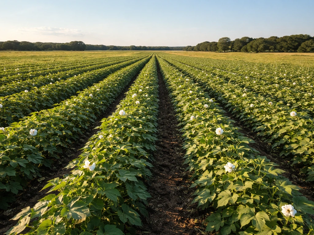
Cotton was king, and it wasn't a close contest. While Texas planters also grew corn, sugar in coastal areas, and some tobacco, none of those came close to matching cotton's combination of market demand, price per pound, and suitability for the Texas environment. Cotton was a cash crop in the truest sense: it could be shipped, graded, and sold on global commodity markets in a way that corn simply couldn't.
The economics made sense at every level. A planter who could put 20 to 30 enslaved workers into a cotton field could produce hundreds of bales per season. By turning enslaved labor into high-yield cotton production, planters were able to drive the colonial economies through expanding output, exports, and profits. At mid-1850s prices, which ranged roughly from 8 to 12 cents per pound with occasional spikes higher, a 500-pound bale brought real money. Multiply that across hundreds of bales and you start to see how a well-run plantation could generate significant annual income. And because cotton stores relatively well and travels by bale, it was practical to move from inland Texas farms to port towns like Galveston for export.
Land, labor, and credit: how planters built scale
Wealth at this scale required more than just planting cotton. It required access to land in large enough quantities to matter, a labor force that didn't eat into margins with wages, and credit systems that let planters expand before profits fully materialized. Texas planters had all three, though not without risk.
Land acquisition
Texas land was cheap and available in ways that the older Southern states could no longer offer by the 1850s. Headright grants, land patents, and direct purchase from the state gave planters the ability to accumulate hundreds or even thousands of acres at low cost. The river bottom soils along the Brazos and Colorado were particularly attractive because they combined fertility with access to water transport. Planters who moved early claimed the best land and locked in a geographic advantage that compounded over the decade.
Enslaved labor as the economic engine
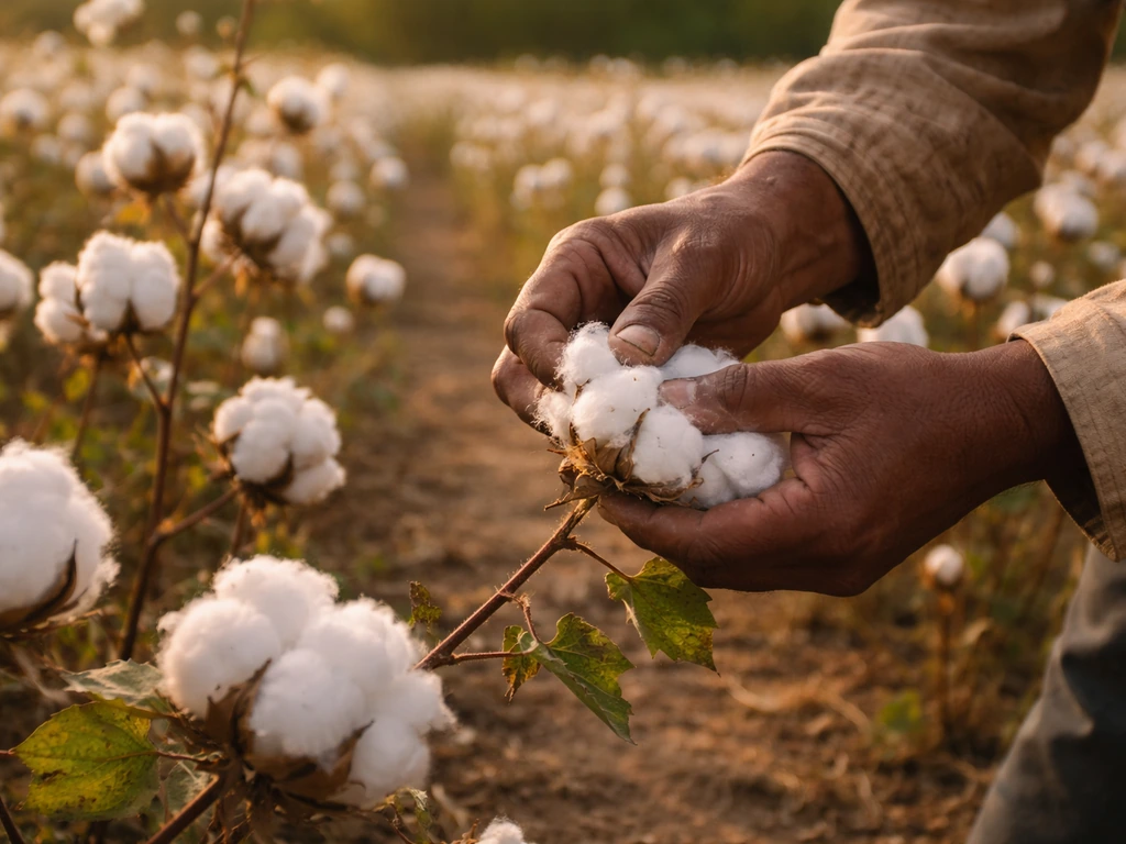
This is where the plantation system becomes inseparable from the profit story. Enslaved people did the planting, cultivating, picking, ginning, and baling. Because planters didn't pay wages, their variable labor costs were mainly food and clothing, which were kept minimal. A planter with 50 enslaved workers could produce at a scale that a free-labor farm of equivalent size simply couldn't match on cost. Enslaved people were also counted as capital assets, listed in wills and tax records alongside land and livestock, so as cotton profits rolled in, planters reinvested in more enslaved workers, which expanded capacity and compounded wealth generation.
Credit and financing
Most planters didn't fund expansion purely from prior-year profits. They used crop-lien arrangements and merchant credit, borrowing against the next harvest to buy land, enslaved workers, and equipment now. Cotton factors (agents in places like Galveston or New Orleans) advanced credit against anticipated bale deliveries, taking a commission when the cotton sold. This system worked beautifully when prices were high and harvests were good, though it also meant planters were exposed to price swings in ways that could turn a bad year genuinely dangerous.
Market connections: moving cotton from field to buyer
Growing cotton was only profitable if you could get it to buyers at the right price. Texas planters benefited from several market linkages that made this feasible, even before the state had an extensive rail network.
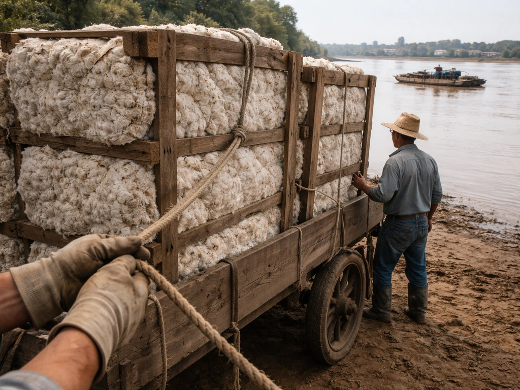
Galveston was the critical export hub. Cotton baled on Brazos and Colorado river plantations moved by wagon or river transport to Gulf Coast ports, where it was loaded onto ships bound for New Orleans, New York, or directly to Liverpool. British textile mills were the ultimate buyers for much of this cotton, and the insatiable appetite of the Lancashire mills kept demand strong throughout most of the 1850s. Rail lines were beginning to extend inland from the coast during this decade, which progressively cut transportation costs and opened up areas further from navigable rivers.
Price cycles did create real volatility. The 1857 financial panic caused a sharp dip in cotton prices, squeezing planters who were carrying debt. But the broader 1850s trend was favorable, and planters who survived the dip generally recovered by decade's end. The key insight is that scale helped: a large planter with 300+ bales had more room to absorb a bad price year than a small operator with 30 bales.
The role of slavery and the plantation labor system
It's impossible to explain planter wealth in 1850s Texas without being direct about this: the plantation system ran on enslaved labor, and that labor is what made the profit margins work. This wasn't incidental to the wealth creation; it was structural. The 1850 and 1860 slave schedules in the federal census document the growth of the enslaved population in Texas cotton counties alongside production growth, and the correlation is not subtle.
Enslaved workers were valued in estate records at prices ranging from roughly $800 to over $1,500 per person by the late 1850s, meaning a planter with 50 enslaved workers held $40,000 to $75,000 in human capital on paper, in addition to land and equipment. This capital could be mortgaged, inherited, and transferred, making it a central pillar of planter wealth accumulation. The broader economic injustice of this system is worth holding alongside the profit mechanics: the people doing the work were the ones denied its fruits.
Understanding how enslaved labor intersected with crop profitability also connects to broader patterns worth exploring, including how commercial crop economics shaped labor arrangements across different historical periods and regions.
Environmental and geographic advantages for cotton cultivation
From a pure crop-growing standpoint, central and coastal Texas in the 1850s was well-suited for upland cotton. The key environmental factors were:
- Long growing season: The Gulf Coast climate gives Texas a frost-free window of 240 to 270 days in many areas, which cotton needs to mature fully from planting to harvest.
- Heat and sunshine: Cotton is a warm-season crop that needs sustained heat. Texas summers deliver that reliably, with temperatures during critical boll-development months frequently above 85 to 90 degrees Fahrenheit.
- River-bottom soils: The alluvial soils along the Brazos, Colorado, and Trinity rivers are deep, well-drained, and naturally fertile, reducing the need for heavy soil amendment and allowing high-yield planting.
- Moderate but reliable rainfall: Coastal and south-central Texas received enough rainfall during the 1850s growing season to support cotton without consistent irrigation, though drought years were a real risk.
- Flat to gently rolling terrain: Much of the plantation zone was easy to cultivate with horse and mule-drawn implements, lowering the labor cost per acre compared to hillier land.
This combination is exactly what agricultural geographers look for when explaining why a crop concentrates in a specific region. Cotton didn't spread uniformly across Texas; it clustered in the zones where all these conditions overlapped, which is precisely the river-corridor plantation districts documented in the TSHA records.
What planter wealth actually looked like (and its limits)
When census records and estate inventories describe a wealthy Texas planter of the 1850s, the wealth typically shows up in a specific combination of assets: acreage (often hundreds to thousands of acres), enslaved workers (the primary labor force and a major capital holding), cotton gins and processing equipment, livestock, and cash or credit with factors in Galveston or New Orleans. Political power came with it, since large planters dominated county and state government through much of the antebellum period.
But wealth had real limits and risks. Cotton price volatility was the biggest threat. A planter who borrowed heavily against a $12-per-pound forecast and then faced an $8 market could find themselves in serious debt. Crop failures from drought, flooding, or insect damage hit hardest on operations that had leveraged land and credit to expand. The 1857 financial panic showed how quickly credit could tighten. And the entire system was built on a political and legal foundation, the institution of slavery, that would be violently dismantled within a decade, wiping out the labor-capital component of planter wealth almost overnight.
How to dig deeper: finding the evidence yourself
If you want to verify or extend this analysis, the primary sources are more accessible than you might expect. Here's where to look:
- 1850 and 1860 U.S. Federal Census Agriculture Schedules: These county-level records report ginned cotton in bales by farm, letting you trace production growth farm by farm through the decade. Many are digitized through Ancestry, FamilySearch, or university digital collections.
- 1850 and 1860 U.S. Federal Census Slave Schedules: These list enslaved individuals by age and sex under slaveholder names, allowing direct comparison of labor force size with production records from the same county.
- Texas State Historical Association (TSHA) Handbook of Texas Online: The entries for 'Cotton Culture,' 'Agriculture,' and 'Antebellum Texas' provide synthesized data and are good starting points for citing official production figures.
- Galveston port export records: Galveston's export figures for cotton in the 1850s document how much was actually moving through to market, which cross-checks census production numbers.
- Texas General Land Office records: These document land grants and patents, giving you a picture of how acreage was acquired and by whom in specific counties.
- Historical cotton price series: The USDA and various agricultural history publications have reconstructed cotton price data by year, which you can layer over the production figures to estimate planter revenue in any given year.
Pairing census agriculture schedules with slave schedules and land records for the same county and planter name is the most powerful method for understanding individual planter wealth. The 1850 federal agricultural census agriculture schedule specifically used “Ginned Cotton” in bales as a reporting field, enabling direct extraction of cotton output from 1850-era production records. You can literally watch a planter's cotton output, enslaved labor force, and land holdings grow in parallel across the two census years.
Comparing the 1850s advantage to other crop systems
| Factor | Texas Cotton Planters (1850s) | Tenant Farmers (same era) | Small Subsistence Farmers |
|---|---|---|---|
| Primary crop | Cotton (cash crop) | Cotton or mixed crops | Corn, vegetables, livestock |
| Labor model | Enslaved labor (no wages) | Family + sharecrop arrangements | Family labor only |
| Land scale | Hundreds to thousands of acres | Rented plots (often 20-80 acres) | Small owned or claimed plots |
| Market access | Direct via cotton factors and Galveston port | Through landlord or local gin | Limited, mostly local barter |
| Credit access | Strong (land and labor as collateral) | Restricted (no collateral) | Minimal |
| Wealth accumulation | High (land, labor capital, reinvestment) | Low to none | Subsistence level |
The contrast with tenant farmers and subsistence farmers shows clearly why the planter class pulled away so dramatically in wealth during this period. One key difference was that tenant farmers had limited control over land and credit, which constrained what they could grow. It wasn't just that they grew cotton; it was that they could grow it at scale, finance that scale, and capture the full margin because their primary labor cost was structurally suppressed. That's the engine behind the sevenfold production increase from 1849 to 1859 and the wealth concentration it produced.
FAQ
If cotton prices were volatile, how did large planters avoid going bankrupt after a bad year in the 1850s?
Large operators tended to survive because they produced hundreds of bales, giving them more cushion if one shipment or sales period fell in price. They also often had access to renewed merchant credit from cotton factors, but survival depended on having enough equity in land and enslaved labor to secure new terms, not just on the crop itself.
Why didn’t free-labor farms in Texas match planter wealth even if they also grew cotton?
Free-labor farms faced higher variable labor costs because they typically had to pay wages, and they often lacked the same credit and market infrastructure. Even when productivity was similar for a season, differences in labor cost structure and financing meant smaller operators could not expand as quickly or absorb downturns as easily.
How did plantation credit work when harvests or shipments were delayed?
Crop-lien and factor advances were typically tied to expected bale deliveries, so delays from weather, transport bottlenecks, or slow ginning could break the sales timeline. Planters sometimes had to renegotiate schedules with merchants or accept worse terms, which could turn a temporary setback into lasting debt.
What role did ginning and processing capacity play, beyond planting acreage?
Ginning mattered because timely processing turned harvested cotton into bales that could be sold, graded, and shipped. Planters with in-house gins and equipment reduced downtime during peak seasons, lowering the chance that high-quality cotton would miss the best market windows.
Were the richest planters always the biggest landowners, or did other assets matter more?
Often they were among the largest landholders, but wealth also clustered around movable capital and borrowing power, especially enslaved labor, processing equipment, and established relationships with factors. A planter with fewer acres but strong credit access and reliable output could sometimes outperform a larger but under-financed competitor.
How much did the decline or stagnation of rail lines inland limit wealth growth compared with river transport?
Rail expansion helped, but wealth initially relied heavily on river corridors and port connections through wagon and steamboat routes. If a plantation was too far from reliable transport, it had higher costs to move bales and greater exposure to missed delivery windows, which could reduce net profit even with good yields.
Did all Texas cotton counties benefit equally from the boom, or did wealth concentrate in specific zones?
Wealth concentrated where multiple advantages overlapped, especially fertile river-bottom soils and dependable access to export routes like Galveston. Counties with weaker soil conditions or poorer transport access tended to have lower yields and higher per-bale costs, slowing wealth accumulation relative to the core districts.
What happened to planter wealth when a credit-heavy operation faced both low prices and a bad crop year?
That combination was the most dangerous scenario because it attacked both sides of the business model, lower revenue and higher fixed commitments. When a planter had borrowed heavily against a forecast, drought, flooding, or insect damage could prevent repayment, forcing foreclosure or the sale of assets to settle debts.
Why was the 1857 financial panic such a turning point for cotton planters?
The panic tightened credit and pushed down cotton prices, which hit planters who were already carrying debt. Even if demand abroad remained strong later, the immediate issue was financing, lenders and factors became more cautious, and some planters had to accept unfavorable terms to stay afloat.
How can you use census records to tell whether wealth came more from land, labor, or credit in an individual case?
Compare changes between the relevant census years in acreage, enslaved population, and cotton output alongside any recorded assets like livestock and equipment. If output rises alongside enslaved labor and acreage, with consistent improvements in processing capacity, that points to investment-driven growth; if output drops while debt remains high, credit exposure likely drove risk and outcomes.
Did political power increase planter wealth, or was it mostly a result of wealth?
It worked both ways. Wealth gave planters influence in county and state politics, which could help preserve favorable legal and economic conditions, while political connections could also improve access to information and credit relationships. This feedback loop made it harder for smaller farmers to compete for land and market advantages.
If you want to understand the wealth story without focusing only on cotton output, what should you look at next?
Track how planters converted harvests into cash, the timing and terms of sales through factors, and whether they reinvested by expanding enslaved labor or equipment. Looking at estate inventories and mortgage or lien patterns can reveal whether wealth accumulation was primarily reinvestment-driven or debt-driven.
Next Articles
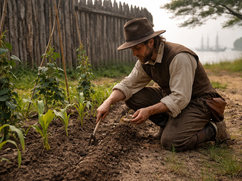
What Did Jamestown Grow and How They Farmed It
Learn what Jamestown colonists grew and the methods they used to plant, harvest, and adapt crops to Virginia conditions.
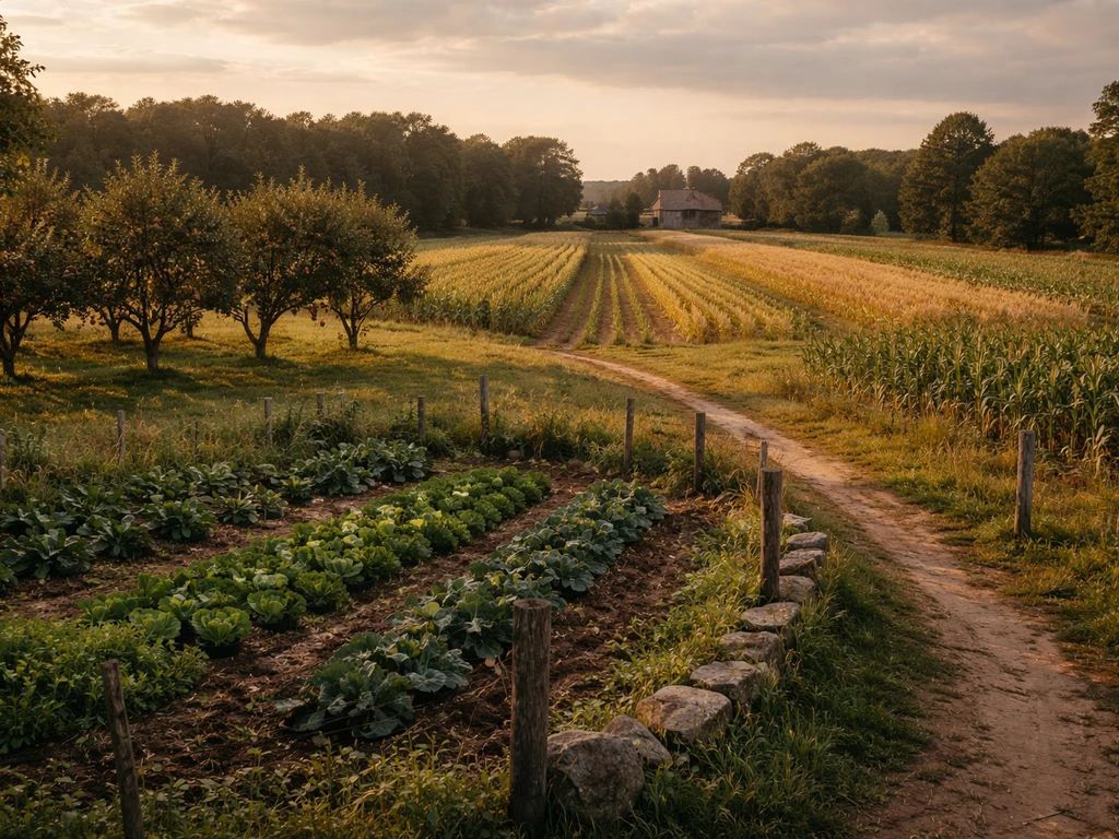
What Did the New England Colonies Grow? Major Crops
Major New England colonial crops explained by climate and soil, from corn and wheat to beans and hay, plus today’s paral
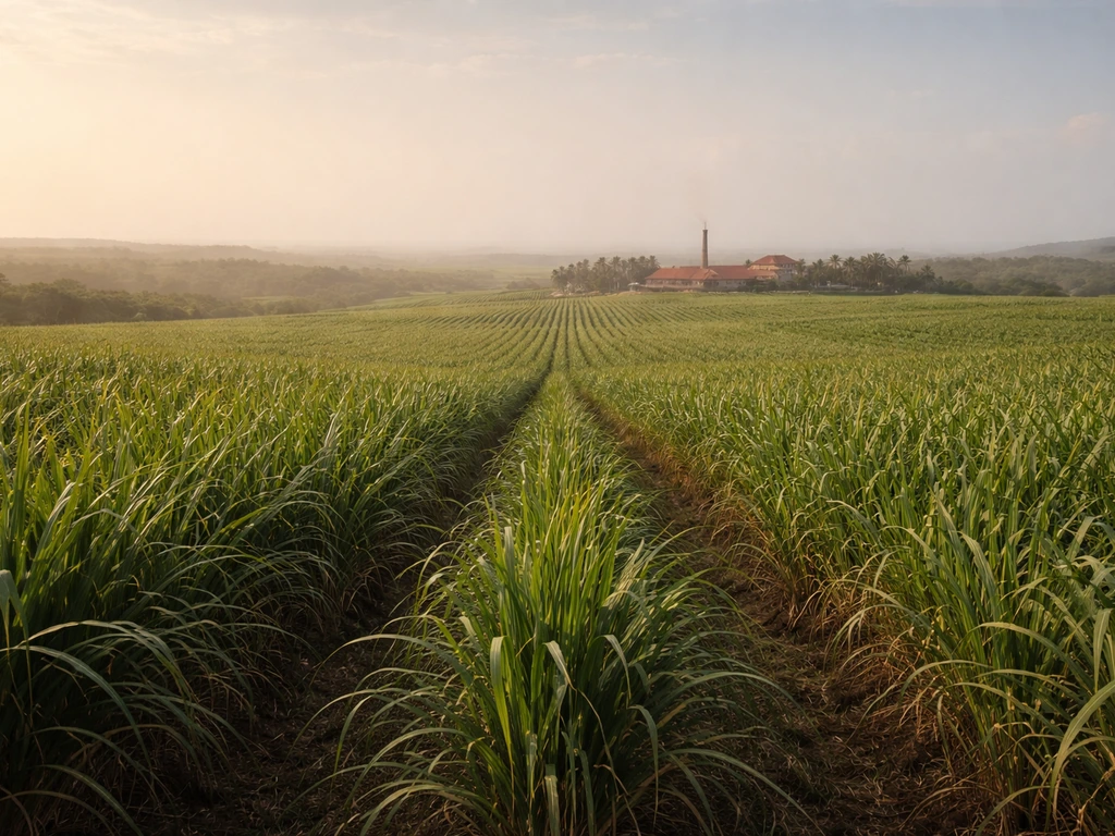
What Europeans Mostly Grew in Caribbean Colonies
Learn which crops Europeans dominated in Caribbean colonies, especially sugarcane, plus key supporting estate plants by